The absolute flux calibration of CASSIS and IDEOS spectra is described in Lebouteiller et al. (2011) and relies on truth spectra published in IRS Technical Report 12003.
What can we learn from repeat observations of the same object about how well the absolute flux calibration works out in practice? How well can the spectral slope and features be reproduced from one observation to the other? Are they the same within the RMS uncertainty of the observation?
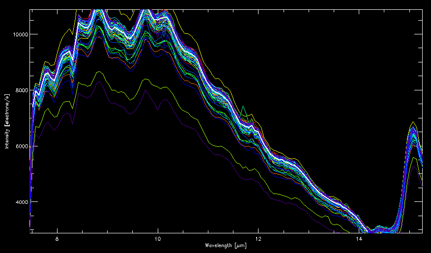
Below we show 81 re-observations of the same calibration star (HD
173511) in the exact same observing mode (SL order 1, nod2).
The SL1 spectra are shown in raw form (extracted from DROOP-corrected
images), in units electrons/s, i.e. before flux
calibration. Clearly the spectra do not fall on top of each
other within the RMS uncertainty of the observations.
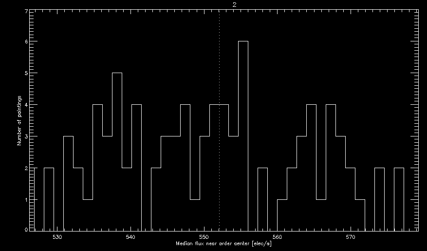
The histogram underneath the
spectrum shows this in a more quantitative way. Ignoring the two
outermost points in the distribution of fluxes measured at a
mid-order reference wavelength, the remaining observations
are scattered over a 6% range in flux.
As can be clearly seen
the distribution is not gaussian. There is a long tail extending
to lower fluxes, indicative of flux losses due to slight mispointings.
According to
Figure
9.4
of the Spitzer
IRS Instrument Handbook v5.0, 27% of
observations of calibration stars have mispointings of 0.36" to 0.62",
which is large compared to the width of the slit: 3.6". Especially in
SL1 where the PSF is fatter than in SL2.

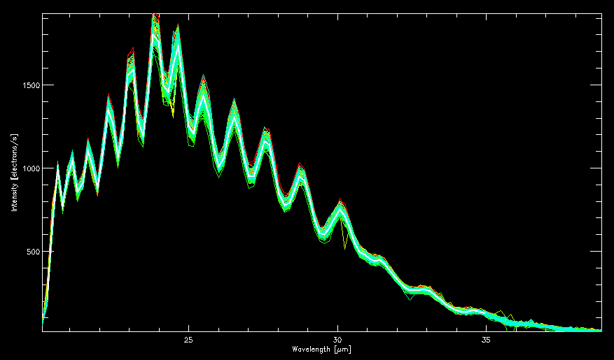
Below the same plots for observations conducted in LL1 nod2. The distribution of fluxes is different than for SL1: no asymmetry. Excluding the two most extreme measurements the spread is 9% with a 1-sigma scatter of 3%. The absence of a tail at lower flux levels indicates that mispointings are not an issue affecting LL1 observations. This is not surprising given that most mispointings (68%) are less than 0.36 arcseconds (Figure 9.4 of the Spitzer IRS Instrument Handbook v5.0),which is small in comparison to the LL slit width.
The above analysis of repeat observations of calibration stars shows
that no two observations of the same object are likely going to turn
out the same: the absolute flux can differ by a few percent based on
the magnitude of the mispointing.
For bright sources, like calibration stars, source acquisition and centering
can be performed at the highest
accuracy level. For dimmer sources this process may not be as accurate.
Below we will show repeat observations of several fainter 'red calibrator'
sources. Unlike the calibration star observations, which we showed
as DROOP-level data (i.e. before the flux calibration step in the IRS pipeline),
these spectra were extracted from the final BCD (basic calibrated data) images,
used by the extraction alogorithm of CASSIS
for their spectral database.
[Note that IDEOS spectra are derived from these CASSIS spectra and differ by only
three addionional enhancements: 1. lining up of the spectral segments by scaling
the spectral segments. 2. Stitching them together by removing the
order overlaps. 3. Applying a redshift correction to obtain the
rest frame spectrum.]
The table below summarizes our findings for the repeatability of an observation for three 'red calibrator' galaxies. The percentages shown in the table indicate the 1-sigma scatter of the spectra around the mean for each of the galaxies and four spectral segments. For all three galaxies the biggest scatter is found for the SL1 segment. This is not surprising because in SL order 1 (7.5-14$microm) the PSF is large compared to the width of the slit. A small pointing error suffices for significant flux loss.
Conclusion: the absolute flux levels of a CASSIS spectrum cannot be known to better than a few percent. Scaling, as needed to turn a CASSIS spectrum into an IDEOS spectrum, introduces additional uncertainties. These are discussion on our aperture corrections info page.
The results for each of the three red calibrator galaxies are given below the table.
| Repeat observations of science targets: sigma/mean | |||
| Integration range | Mrk 231 (16 obs) |
IRAS 07598 (12 obs) |
IRAS 08572 (9 obs) |
5.5-6.5µm (SL2) | 1.4% | 0.8% | 1.3% | 8.5-9.3µm (SL1) | 3.1% | 5.0% | 2.7% | 14.5-15.4µm (LL2) | 2.1% | 1.8% | 1.4% | 23-25µm (LL1) | 2.0% | 2.1% | 1.1% |
In the figure below we have plotted 16 repeat observations of the red calibrator source Mrk 231 taken from CASSIS. The IDEOS IDs for these observations are: 13731584_0, 17102592_0, 17202688_0, 17206272_0, 19318016_0, 21099776_0, 21110272_0, 21453568_0, 22157312_0, 24727808_0, 24915456_0, 27017728_0, 27382272_0, 27749888_0, 34294016_0, and 4978688_0. The spectral segments are as-observed (i.e. they have not been scaled). Apart from the order 1 and 2 segments we include the 'bonus' order for each of the modules (SL and LL). The bonus order segments are used to align (scale) the spectral segments but are not otherwise included in the final IDEOS spectra.
As can be clearly seen, the repeat observations do not lie on top of each other within the RMS uncertainties of the observations. At 24 microns the difference in flux between the highest and lowest spectrum amounts to 7.5% with a 1-sigma scatter of 2.0%. At 15 microns this amounts to 7.8% with a 1-sigma scatter of 2.1%.

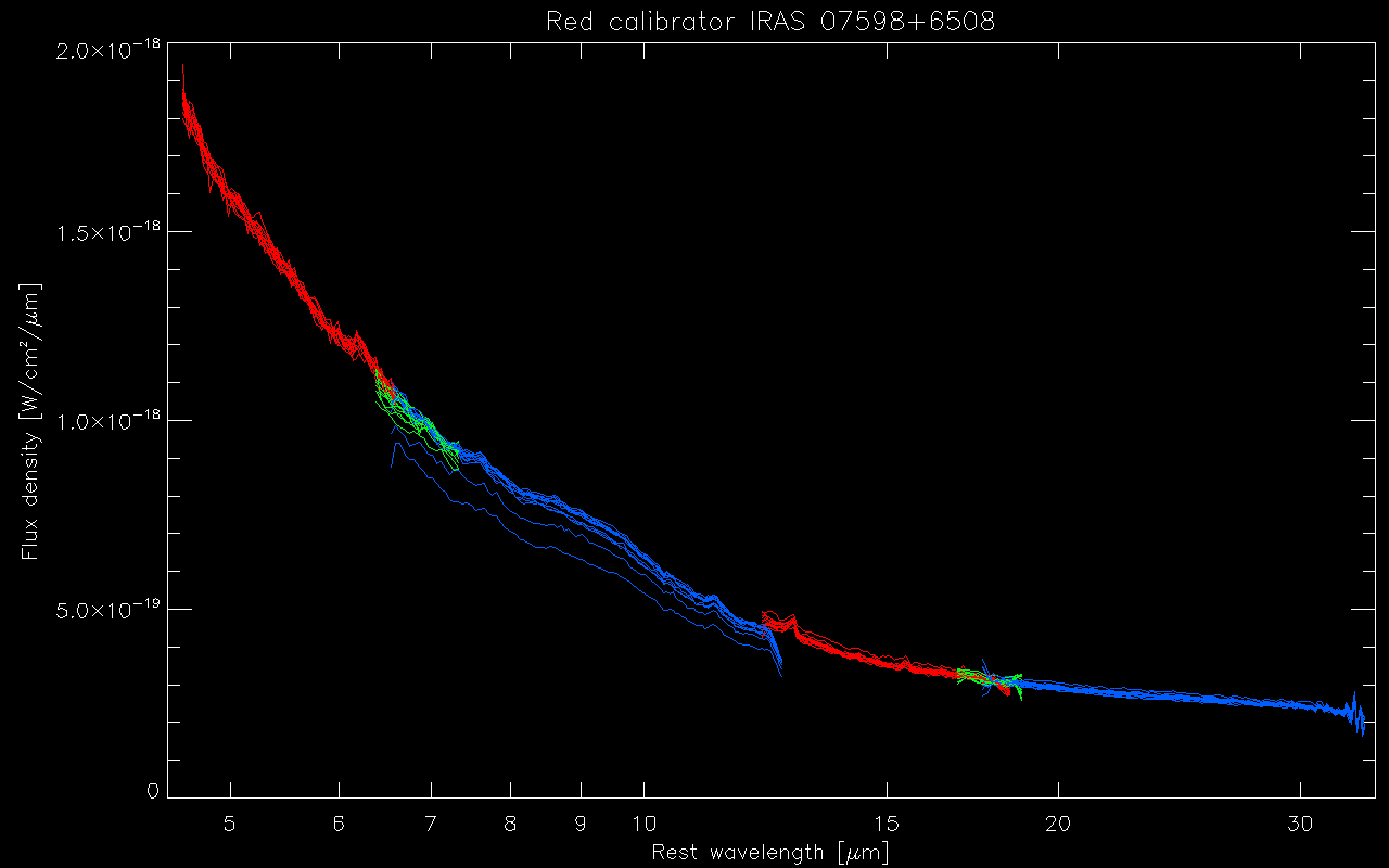
In the figure below we have plotted 12 repeat observations of the red calibrator source IRAS 07598+6508 The IDEOS IDs for these observations are: 17103104_0, 20697344_0, 21457664_0, 24377600_0, 24567296_0, 27015680_0, 28576768_0, 28703744_0, 32514304_0, 33776640_0, 4971008_0, and 7840768_0. Note the two repetitions of the SL1 spectral segment that are significantly offset from the other repetitions. In these observations the source was likely not well centered in the SL slit.
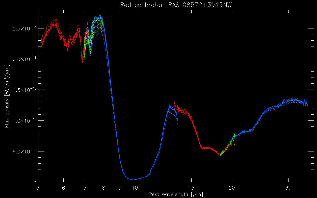
In the figure below we have plotted 9 repeat observations of the red calibrator source IRAS 08572+3915. The IDEOS IDs for these observations are: 16459520_0, 20925696_0, 21457920_0, 24568064_0, 27017216_0, 27381760_0, 28704256_0, 34293504_0, and 4972032_0. One SL1 spectrum shows significantly lower flux than the rest. The source is likely not well-centered in that repetition.
Many galaxies are extended or semi-extended compared to the PSF of Spitzer-IRS. For these galaxies not only the former but also the latter problem may affect the measured flux.
A low-resolution full spectrum is obtained in the following order. At each step pointing errors may be incurred, which compound through step 9: