The width of the LL slit (14-36µm) is bigger than the width of the SL
slit (5-7.5µm): 10.2 versus 3.6 arcseconds. This means that for
(semi-)extended sources, such as galaxies, a larger fraction of the
source will fall within the LL slit than within the SL slit.
To give an example: At z=0.09 the SL slit will record light from the
inner r=3 kpc, and the LL slit from the inner r=8.6 kpc around the nucleus.
At z=0.30 these numbers are r=8 kpc (SL) and r=23 kpc, respectively.
The SL and LL slits are also almost orthogonal to each other. In the dispersion direction the SL slit thus covers a different part of a galaxy than the LL slit does.
Because of the different aperture sizes, stringing together a SL and LL spectrum of an extended source will result in a jump in flux at the stitching wavelength (14.0-14.2µm observed wavelength), with the higher flux occuring in the LL spectral segment.
For the purpose of spectral decomposition or spectral fitting an aperture correction is needed to remove the jump. In IDEOS we chose to scale up the SL spectral orders to match the LL ones, resulting in median correction factors of 1.16.
How do we stitch? As explained in our Paper I, Hernán-Caballero et al. (2016), MNRAS, 445, 1796, we use the small overlap between orders (SL1 and SL2; LL1 and LL2) and between modules (SL1 and LL2) to match the continua in both spectral segments. At some redshifts the order or module overlap occurs in a spectral feature. For instance a PAH feature: e.g. the PAH127 feature at redshifts z=0.10 to z=0.14. For these sources we have no choice but to match the continuum+PAH emission in both segments.
The implicit assumption in applying the aperture correction is that
the source properties as probed in the bigger LL slit are the same
as in the smaller SL slit. While this may be true for some diffuse
extended galactic
objects, this will not be true for galaxies. The LL spectrum will
have a larger contribution from the galaxy disk than the SL spectrum
does. Only above z=0.3 this problem will go away, as even the SL
will probe a radius of r=8 kpc around the nucleus. At z>0.3, a
SL scaling factor above unity thus implies an issue with the
centering of the source in the SL slit.
Note that galaxies in an advanced stage of merging are far more
compact than normal (starburst) galaxies. Some appear as point
sources for Spitzer-IRS. Galaxies like these will not require
aperture corrections as large as other galaxies at the same
redshift.
What are the practical implications of an aperture correction?
It depends. Remember the implicit assumption in the scaling of SL to LL:
the source properties as probed in the bigger LL slit are the same
as in the smaller SL slit. For a coronal line originating from the
AGN point source it is hard to argue that this line would be similarly
distributed within the SL slit as within the LL slit. Luckily, the
main mid-infrared AGN tracers 14.32 & 24.32µm [NeV] and 25.89µm [O IV]
all fall in the LL spectral range even at z=0 and hence do not require
any scaling.
For lower excitation lines like 12.81µm
[NeII] it is easier to argue that they also contribute outside the SL
slit within the LL slit width, as HII regions are found along spiral
arms and bars. On the other hand, even for these lines
the flux is likely concentrated where most of the star formation
occurs: towards the nucleus.
The reality thus may be that spectral scaling distorts a diagnostic
line ratio that is composed of a line in SL and a line in LL by 2-20%
and even higher for nearby galaxies. This distortion should always be kept
in mind when interpreting subtle differences among galaxies, or
between an observed and a model ratio.
Only for higher redshift sources the spectral features residing in the
5 to 14µm range will shift into the LL module one by one: at z>0.1
both lines in the [NeV]/[NeII] and in the [NeIII]/[NeII] ratio will
be observed in the LL
orders. And at z>0.35 also both lines of the [S IV]/[S III] ratio.
The plots below are intended to give an indication of what redshift
ranges are sweetspots and what wavelength ranges require attention for
the correct interpretation of a line ratio.
The scaling factors applied to the spectral segments of a spectrum are listed in the header of each IDEOS spectrum, and can also be found in the 'SED' tab of a single source results page in the IDEOS portal.
Each scaling comes with an uncertainty, which propagates to shorter wavelengths. If, for instance, the SL1-LL2 scaling cannot be pinned down to better than a factor 1.03 to 1.08, this uncertainty propagates to the rest of the SL spectrum. If on top of that the SL2 scaling relative to SL1 falls between 1.01 and 1.03, the uncertainty in the absolute flux in the SL2 spectral segment ranges between 1.03x1.01 on the low end and 1.08x1.03 on the high end. This means that the integrated flux of a feature in SL2 will have a systematic uncertainty of 4% to 11% in addition to the uncertainty computed in the fit. Equivalent widths, optical depths and crystalline silicate strengths are not affected by this.
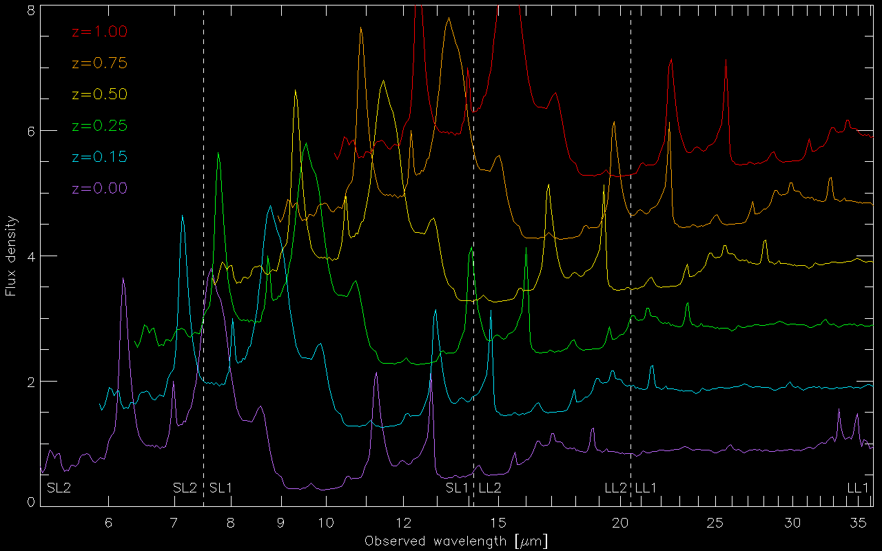 This graphic shows how the mid-infrared spectrum of a Seyfert galaxy
moves through the SL and LL slits and spectral orders as a function of
redshift. Whereas the PAH62, PAH77, PAH86, PAH112 and PAH127 features
all fall within the SL spectral range at redshifts below z=0.09,
the PAH112 and PAH127 features have shifted into the wider LL slit
above z=0.3.
This graphic shows how the mid-infrared spectrum of a Seyfert galaxy
moves through the SL and LL slits and spectral orders as a function of
redshift. Whereas the PAH62, PAH77, PAH86, PAH112 and PAH127 features
all fall within the SL spectral range at redshifts below z=0.09,
the PAH112 and PAH127 features have shifted into the wider LL slit
above z=0.3.
 This diagram shows how commonly observed
mid-infrared emission features shift through the two spectral order
segments of the SL and LL slits as a function of redshift.
The LL slit is much wider than the SL slit. For (semi-)extended
sources the flux density observed thus depends on
whether the continuum, line or feature was observed in the SL or
the LL slit.
This diagram shows how commonly observed
mid-infrared emission features shift through the two spectral order
segments of the SL and LL slits as a function of redshift.
The LL slit is much wider than the SL slit. For (semi-)extended
sources the flux density observed thus depends on
whether the continuum, line or feature was observed in the SL or
the LL slit.